code
Adding KV caching to Karpathy's gpt.py by hand
1. What I wanted to understand
I worked through Andrej Karpathy’s walkthrough on building a GPT. I had no prior exposure to transformers or language modeling; I’d used models, but wanted to understand the innards of a simple one.
From model cards and popsci explanations, I had gathered that transformers use attention heads, that a head calculates the “relevance” of each token to every other token (now I know this is called attending to past tokens), and that this relevance is then used by a feedforward network to get scores over a token vocabulary, which are converted into probabilities and sampled for the next token. But I was pretty hazy on how any of this is calculated, and I’d heard terms like KV caching thrown around, so I decided to swallow the frog.
I also wanted a break from my usual workflow: spinning up worktrees (Conductor) with two or three prompts and getting handed diffs to review, most of which I couldn’t really read. This time I wanted to understand the data flow, keep things simple, write most of the changes by hand, and get a refresher on tensors and GPU execution along the way.
The starting point was Karpathy’s Let’s build GPT video and its repo, karpathy/ng-video-lecture.
KV caching felt like the right size of project: it’s the thing everyone mentions when talking about inference, Karpathy’s generate doesn’t have it, and adding it means touching every layer of the model (heads, blocks, the top-level forward and the sampling loop), so I’d have to actually understand the data flow instead of nodding along. I expected to stop recomputing keys and values for tokens the model had already seen, and mostly wanted to find out whether I could get the tensor shapes right without someone handing me the diff.
Source links: Karpathy source · my implementation · diff
Setup: Karpathy’s config, unchanged: 6 layers, 6 heads of size 64 (n_embd = 384), a 256-token context, a 65-character vocabulary, about 10.8M parameters, float32. Run on an Apple M5 with 24 GiB of RAM.
1a. A quick refresher on the nanogpt architecture
I learned most of this for the first time, so here’s my understanding of the transformer, written down.
Tokens
Take a short sentence and split it two ways:
"The cat eats fish"

words:       The · cat · eats · fish                               4 tokens
characters:  T·h·e·␣·c·a·t·␣·e·a·t·s·␣·f·i·s·h                     17 tokens
Words give short sequences, but the vocabulary would be immense (the Oxford dictionary has about 600k entries, from a quick search). Characters give a tiny vocabulary (under 100), but sequences about 4× longer. Modern tokenizers like OpenAI’s tiktoken split the difference with subwords (byte-pair encoding: frequent character chunks of varying length). For simplicity, nanogpt uses characters.
An embedding table turns each token, like t, into a vector. So the input to the transformer is a tensor X of shape (B, T, C): B = batch size, T = number of tokens (time), C = embedding size. I like to think of it as B sentences of T words each, with every word represented by a feature vector of length C.
So far, the tokens don’t know where they sit in the sentence: a verb can’t tell whether it’s at the beginning or the end. So nanogpt also adds a positional embedding to every token. This is a second learned table, position_embedding_table, with one row per absolute position 0..255 (not the sine/cosine encoding from the paper). This matters later.
Attention
The core idea from “Attention Is All You Need”: given the current tokens and how relevant they are to each other, which tokens should contribute to each token’s information, and how much? nanogpt answers that with three linear projections of x, the query, key and value. Here is one head from Karpathy’s code:
k = self.key(x)   # (B,T,hs)
q = self.query(x) # (B,T,hs)
# compute attention scores ("affinities")
wei = q @ k.transpose(-2,-1) * k.shape[-1]**-0.5 # (B, T, hs) @ (B, hs, T) -> (B, T, T)
wei = wei.masked_fill(self.tril[:T, :T] == 0, float('-inf')) # (B, T, T)
wei = F.softmax(wei, dim=-1) # (B, T, T)
wei = self.dropout(wei)
# perform the weighted aggregation of the values
v = self.value(x) # (B,T,hs)
out = wei @ v # (B, T, T) @ (B, T, hs) -> (B, T, hs)hs is the head size: C divided by the number of heads, so 384 / 6 = 64 here. The heads’ outputs are concatenated back to (B, T, C).
wei is a (B, T, T) matrix of how much token i attends to token j. To keep it causal (a token can’t attend to future tokens), everything above the diagonal is set to −∞ before the softmax. For three tokens, the weights after the softmax look something like:
[[1.0, 0.0, 0.0],
 [0.8, 0.2, 0.0],
 [0.5, 0.2, 0.3]]
Each row sums to 1, so wei @ v gives every token a weighted sum of the value vectors of itself and the tokens before it. The k.shape[-1]**-0.5 factor (1/√hs) keeps the variance of the dot products in check, so the softmax doesn’t saturate.
That’s all math, but what do these projections mean?
- Query: what am I (the token) looking for? If tokens were words, “eats” as a verb is looking for a subject, like “cat” or “man”.
- Key: what do I have to offer someone who’s looking? “cat” would hold a learned representation that can be found by something looking for a subject noun.
- Value: what do I actually pass on? If “eats” attends to “cat”, this is the information that gets sent forward.
The rest of the block
nanogpt uses attention in a residual manner, followed by a feedforward network, with a LayerNorm before each:
x = x + self.sa(self.ln1(x))
x = x + self.ffwd(self.ln2(x))Per Andrej, the residual path helps gradients flow and offers a way to effectively skip a block, which helps in deeper networks. The feedforward network transforms the features within each token. After the last block, the output is turned into logits over the vocabulary, then into a probability distribution to sample the next token from.
2. What I changed
nanogpt was a great primer for getting a no-nonsense transformer up. But its generation loop recalculates everything for every new token. This is Karpathy’s loop:
for _ in range(max_new_tokens):
    # crop idx to the last block_size tokens
    idx_cond = idx[:, -block_size:]
    # get the predictions
    logits, loss = self(idx_cond)
    # focus only on the last time step
logits = logits[:, -1, :] # becomes (B, C)Every step runs the whole context through the whole model, then throws away all but the last row of logits. For example, k = key(x) gets computed for x of shape (B, T+1, C), even though the previous step already computed it for the first T tokens.
When “fish” is the new token, we don’t need the queries for “the”, “cat” and “eats”, but we do need their keys and values:
new token:   fish
compute:     q_fish, k_fish, v_fish
reuse:       k_the, k_cat, k_eats   →  attention weights for "fish"
             v_the, v_cat, v_eats   →  output o_fish
Old queries are useless because a query only computes its own token’s output, which was already done and, with a causal mask, never changes. Keys and values get read by every future query.
That’s the concept behind KV caching: prefill K and V for the previous tokens once, then during decode pass only the new token through the q, k, v projections. Each head keeps its K and V in memory, and the computation that was redundant for previous tokens goes away.
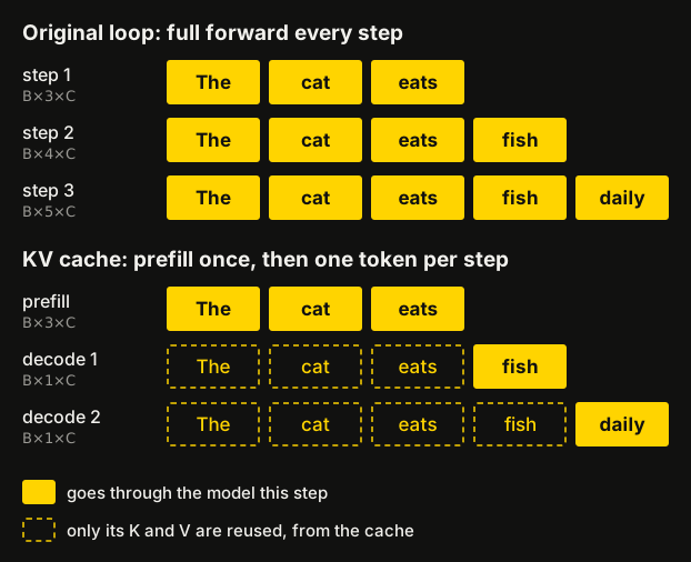
Figure 1. Words as tokens for readability; the real model uses characters.
So generation splits into two phases. Prefill runs the prompt through the model once and every head hands back its K and V. Each decode step then pushes only the sampled token through, with the cache:
logits, _, cache = self(idx, past_kv=None)

# idx is (B, T) array of indices in the current context
for step in range(max_new_tokens):
    logits_last =logits[:, -1, :]
    probs =F.softmax(logits_last, dim=-1)
    idx_next = torch.multinomial(probs, num_samples=1) # (B, 1)
    # append sampled index to the running sequence
    idx = torch.cat((idx, idx_next), dim=1) # (B, T+1)

    if step ==max_new_tokens -1:
        break
logits, _, cache = self(idx_next, past_kv=cache)Inside each head, the new token’s k and v get appended to the cached ones along the time axis:
k = self.key(x)   # (B,T,hs)
q = self.query(x) # (B,T,hs)
v = self.value(x) # (B,T,hs)
if past_kv is not None:
    k_past, v_past = past_kv
    k = torch.cat([k_past, k], dim=1)
    v = torch.cat([v_past, v], dim=1)
# ...
return (out, (k,v))The cache is threaded through the model as nested lists, past_kv[layer][head] = (k, v), so 6 × 6 × 2 = 72 tensors of shape (B, T_total, 64). torch.cat is the simplest option, but it copies the whole cache on every step; preallocating (B, block_size, 64) buffers would avoid that. Attention itself still grows with context, since the newest query is dotted against every cached key.
3. How I checked it
Since caching only skips work, it shouldn’t change the math: for the same weights and tokens, the cached model has to produce the same logits as a full forward, up to float rounding. check_kv_cache.py checks exactly that, against Karpathy’s original model with the same weights loaded, so my changes aren’t on both sides of the comparison.
| Check | Max abs diff (CPU / MPS) | Result |
|---|---|---|
| Full forward, N = 1 to 256 | 0 / 0 | pass |
| Prefill N−1, then one cached token | ≤ 1.1e-6 / ≤ 9.9e-7 | pass |
| Decode one token at a time up to 256 | ≤ 1.8e-6 / ≤ 1.7e-6 | pass |
| Prefill, then a chunk of several tokens | ≤ 1.4e-6 / ≤ 1.4e-6 | pass |
| Greedy generation, 200 tokens × batch 2 | — | 400 / 400 identical |
Random (untrained) weights, eval() + no_grad, float32; pass means allclose(atol=1e-5). To make sure that threshold isn’t hiding anything, I broke the cached path on purpose (skipping the position offset, or the mask offset for multi-token chunks): the differences jump to about 1. eval() matters because dropout (0.2) would otherwise draw different masks in the two runs.
So with dropout off, the cached path matches Karpathy’s original to float noise. What this doesn’t cover is trained weights.
4. What I traded away, and what I would try next
Currently there’s no sliding window, so generation is capped at 256 tokens in total: I ran out of energy before implementing the sliding window by hand. It isn’t as simple as dropping the oldest token’s k and v. nanoGPT uses learned absolute positional embeddings, and the original generation loop resets token positions whenever it crops the context, so the cached entries would go stale in two ways: every kept token’s old absolute position is baked into its K/V in every layer, and from the second block onward its K/V were computed while the evicted token was still in context.
The easiest approach would be to cache until we hit the context window, then discard the cache and rebuild it from the latest tokens, sort of like a sawtooth wave. Not from the full latest 256, though, or it overflows again on the very next token; something like the last 128.
The next thing I’d try is that sawtooth window, and checking how soon its output diverges from the original crop-and-recompute loop past the 256 mark. After that, rerun the equivalence checks on trained weights.
Disclaimer: I used Claude Code to write the logit check script, draw the figures, and edit this note (formatting, a few technical corrections, and some of the connecting paragraphs). The KV cache implementation is mine.