Tractor telemetry at Carnot - some tractors never leave the village, others cross state lines

Context before this came up

Carnot Technologies was founded in 2015 by four IIT Bombay alumni from the IIT Bombay Racing team, where they had built systems to monitor race-car performance. The company later moved into agricultural technology, building connected hardware and software for tractors and other farm equipment. Mahindra & Mahindra invested in Carnot and raised its stake to about 69% in 2022. By FY2023, Carnot had deployed nearly 30,000 Krish-e Smart Kits across India.

The Smart Kit was essentially a GPS tracker with a wiring harness that could be retrofitted to tractors from different manufacturers. Owners could see in a mobile app where a tractor was, how long it had been running, how much land it had worked, and how much fuel it had used. This was particularly useful for tractor rental businesses, where the owner usually isn’t with the tractor.

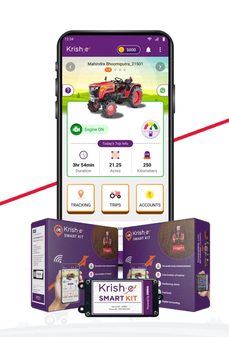The Krish-e Smart Kit and the Krish-e app. Image: Carnot Technologies.

I joined Carnot as a data scientist in August 2024. By then, a lot of telemetry was coming in from tractors across the country. The Smart Kit told individual owners what their tractors were doing. The question I worked on was one level up: what could a tractor manufacturer learn from how thousands of its machines were actually being used?

What can you learn from a tractor?

Some Smart Kits were retrofitted by owners. Others were installed by original equipment manufacturers (OEMs), sometimes before the tractor had left the factory, which gave the manufacturer a view of its machines well beyond the point of sale.

An OEM might know how many tractors it sold in Maharashtra, but not what happened afterward. Were they mostly farming or hauling goods? How many hours did they run? Did usage change across seasons? Were certain models used more at night?

The answers varied a lot. Some owners travelled 60 km a week, others more than 300 km. Some tractors worked year-round, others for a couple of months. Some rarely went beyond a 20 km radius, others crossed state boundaries. Sub-40 HP models dominated some regions, while 60+ HP machines were more common elsewhere.

This mattered for product design, not just sales. A tractor hauling goods over long distances faces different demands from one working fields for a couple of months a year. Haulage distances, engine RPM during farming, or hours driven at night could show whether a tractor was designed for how customers actually used it, and reveal customer profiles that sales figures didn’t.

Other questions were more operational: whether customers went to authorised service centres or independent garages, where and how tractors were refuelled, and what battery voltage said about engine activity and battery health. We even looked for highway crossings that might make good billboard locations. OEM-fitted devices also let us follow tractors from factories through depots and warehouses to dealerships, looking for bottlenecks.

The data itself wasn’t exotic: GPS coordinates, timestamps, speeds, and a few sensor readings. The hard part was working out what we could reasonably infer from it, and making that work across thousands of tractors and months of activity.

Two synthetic tractors over June 2025: field work near Baramati (about 260 km) and haulage out of Dewas (about 3,400 km).

Where my work started

Each Smart Kit sent telemetry roughly every one or two seconds: location, speed, timestamp, and sensor readings. A single tractor could generate tens of thousands of readings a day. Across thousands of tractors, even “how much time did tractors spend farming in this district last month?” becomes a real data-processing problem.

The raw telemetry was stored as Parquet files on Amazon S3. Carnot already had Python pipelines that turned these readings into trajectories, trips, farming activity, and estimated acreage for each tractor, so I wasn’t starting from raw GPS coordinates.

My work began one level above that. Instead of what one tractor did yesterday, we wanted patterns across thousands of tractors, over weeks or months, and across geographies. That meant combining device-level data with spatial data, aggregating it over time, and making the results available for analysis.

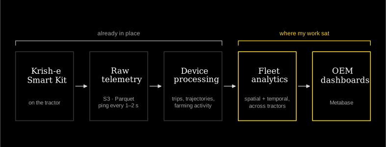From the Smart Kit to OEM dashboards. My work was the last two stages.

DuckDB: when Pandas stopped being enough

Running out of RAM

Most of my analysis started from Parquet files in S3. For small datasets the workflow was simple: read the files into Pandas, filter, group by whatever I was interested in, and compute some statistics.

That stopped working as the datasets grew. One tractor over a few days was fine; thousands of tractors over several months was not. Pandas loads the data into memory, and I regularly ran out of RAM before getting to the interesting part.

The annoying thing was that I rarely needed all the data. Average daily operating hours by tractor model needs a handful of columns and one aggregation. Loading every record into a DataFrame just to throw most of it away seemed wasteful.

Querying the files directly

DuckDB let me query Parquet files with SQL, from inside Python, without loading the whole dataset into memory first. A simplified example (illustrative, not the production code):

# Pandas: load the data, then aggregate
import pandas as pd

df = pd.read_parquet("tractor_activity.parquet")
result = (
    df.groupby("tractor_model")["operating_hours"]
    .mean()
)

With DuckDB:

import duckdb

result = duckdb.sql("""
    SELECT
        tractor_model,
        AVG(operating_hours) AS avg_operating_hours
    FROM read_parquet('tractor_activity.parquet')
    GROUP BY tractor_model
""").df()

The SQL isn’t remarkable. The difference is in how DuckDB runs it: it reads only the columns it needs, processes the data in chunks, and aggregates inside its own engine. I still got a Pandas DataFrame at the end, but it held the small result instead of millions of intermediate records.

It also didn’t need a database server or any extra infrastructure. It’s an embedded engine that runs inside an existing Python workflow, which for exploratory analysis over Parquet files was most of the appeal.

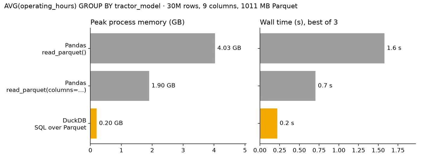Peak memory and time for the same group-by on a 30-million-row Parquet file. Synthetic data, measured on my laptop, not at Carnot.

Enter Uber’s H3

Highways

DuckDB handled most of the number-crunching, but some of the more interesting questions were about geography. Did a tractor spend time on a particular highway? Which districts did it work in? Had two tractors worked the same area?

Take highways. We had tractor trajectories, and highway geometries from OpenStreetMap, so in principle we just needed to find where they intersected.

My first approach used GeoPandas. It worked, but geometric intersections got painfully slow as the number of trajectories grew. And we weren’t asking just once: we wanted to compare activity across highways, districts, seasons, and tractor models, which meant rerunning expensive geometry operations over the same trajectories.

That’s when I started looking at H3, Uber’s open-source geospatial indexing system.

Hexagons

H3 divides the Earth’s surface into a hierarchy of mostly hexagonal cells. Each cell has an ID, and you pick a resolution depending on how much detail you need. An area can then be a set of cell IDs instead of a complicated polygon.

The trick was to do the geographic work once and reuse it. We already had daily trajectories, labelled as farming or commuting. I converted their coverage into H3 cells and stored those next to the activity data. A highway could be represented the same way, by the cells it passes through. Instead of checking whether thousands of trajectories intersect a highway’s geometry, I could compare sets of cell IDs:

# Simplified illustration
tractor_cells = {101, 102, 103, 104}
highway_cells = {103, 104, 105, 106}

overlap = tractor_cells & highway_cells
if overlap:
    print("Possible highway usage")

Real IDs are much longer, but the idea is the same: a geometric intersection often becomes a set operation or a join on cell IDs.

The tradeoff is that sharing a cell doesn’t mean two geometries actually intersect. It depends on the resolution, and cell matches can be false positives. For exploratory analysis and finding candidate overlaps, that was usually acceptable. Where exact boundaries mattered, we fell back to geometry checks.

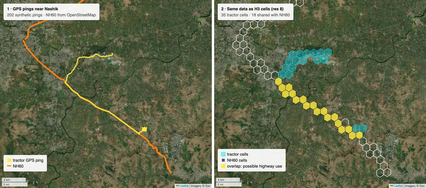Synthetic GPS pings near Nashik (left) and the same pings as H3 cells (right). Yellow cells are shared with NH60.

Districts

The hierarchy helped with another problem: which district a tractor was working in. Coarse cells could quickly identify the likely district, and only points near a district boundary needed an exact point-in-polygon check. That avoided a full lookup for every point without losing accuracy where it mattered.

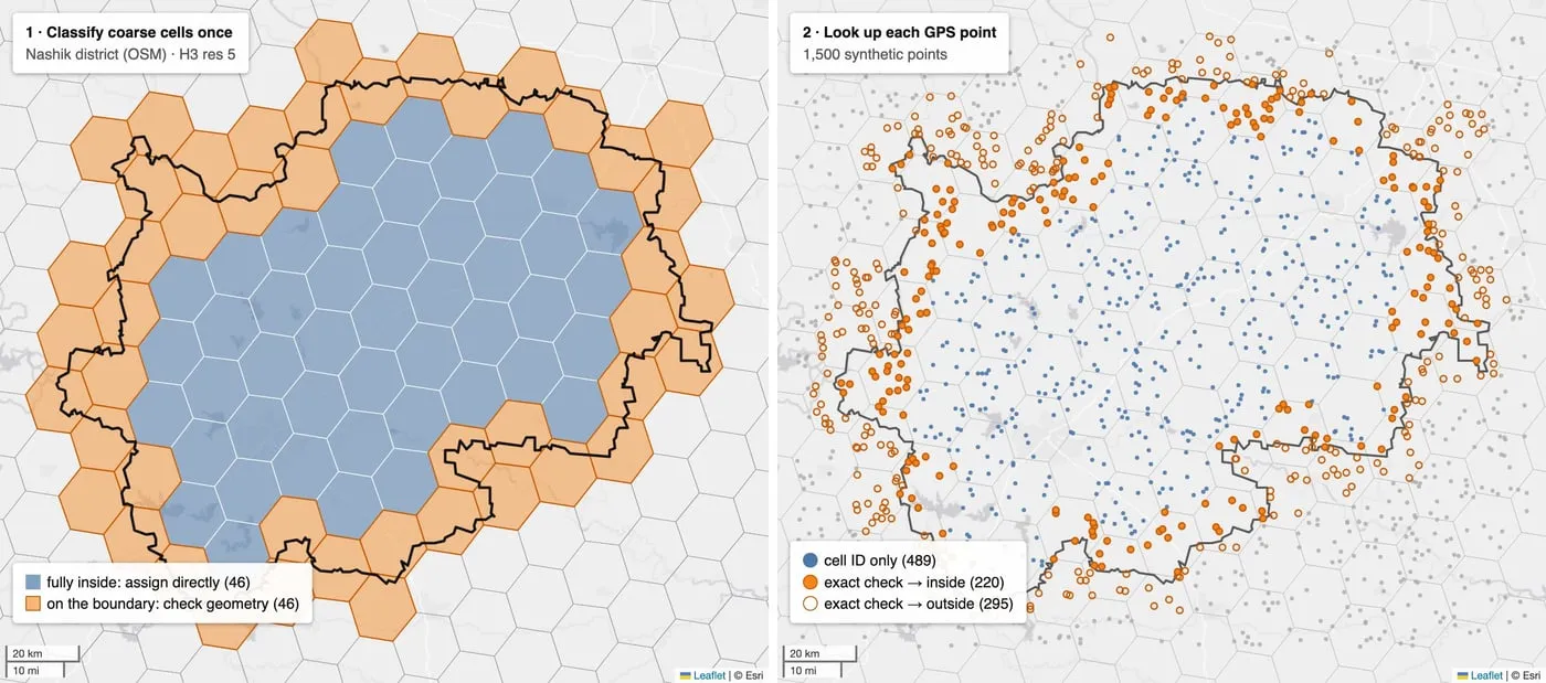Nashik district over coarse H3 cells. Points in interior cells are assigned directly; points in boundary cells get an exact check.

DuckDB also has an H3 extension, so Parquet data, H3 IDs, and SQL aggregations could all live in one workflow.

Hexagons aren’t inherently faster than polygons. What helped was having a precomputed, reusable spatial representation of tractor activity. Once that existed, geographic questions were much easier to write, combine, and rerun.

From my laptop to an OEM dashboard

DuckDB and H3 made it much easier to investigate tractor activity, but answering a question on my laptop isn’t the same as making the answer available to someone at an OEM. A manufacturer might want to compare farming hours across models, filter by district, or see how usage changed month to month, without us answering each question by hand. Ideally, they would open a dashboard, change a few filters, and explore.

We used Metabase for dashboards, with some of the data in PostgreSQL. Over time, the SQL behind the dashboards had become complicated: business logic was spread across nested CTEs and saved Metabase questions, and it was hard to tell which calculations were reused where.

We started moving that logic into SQLMesh, which defines transformations as SQL or Python models, manages the dependencies between them, and materialises datasets for downstream use. The work split into layers: raw and device-level data at the bottom, reusable transformations for activity by tractor, geography, and time period in the middle, and dashboard-ready datasets with the metrics OEMs cared about on top.

Some models reprocessed their entire input, while others updated incrementally as new telemetry arrived. SQLMesh supported both, and its planning workflow made it easier to review changes before applying them.

This separated how a metric was calculated from how someone explored it. Business logic was defined once and reused, instead of being buried inside a dashboard. An OEM shouldn’t need to know anything about Parquet, H3, or SQLMesh to compare how its 40 HP tractors are used in Punjab versus Maharashtra.

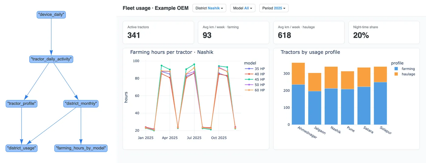A toy SQLMesh project: model lineage on the left, and a dashboard built from its tables on the right.

Looking back

When I joined Carnot, I hadn’t expected to spend so much time thinking about tractor movements, highway intersections, or hexagonal grids. But that’s what made it interesting: a small device sending a few measurements every second could tell us a lot about how tractors were used, if we knew which questions to ask.

None of the tools were complicated to get started with. What I learnt was to understand the input/output requirements and the processing first, and then choose an appropriate tool for each part.

Ad-hoc code often worked (until it didn’t :p), and time and effort went into serving the use case. Telling which use cases needed complex engineering and which could be served by a simple query, and the tradeoffs in each, was not easy for a newbie like me; greenhorns out of college are often attracted to complexity. I had to rethink how I approached a lot of problems, and Carnot helped me get to the ground (literally) and build from there, instead of castles in the air.

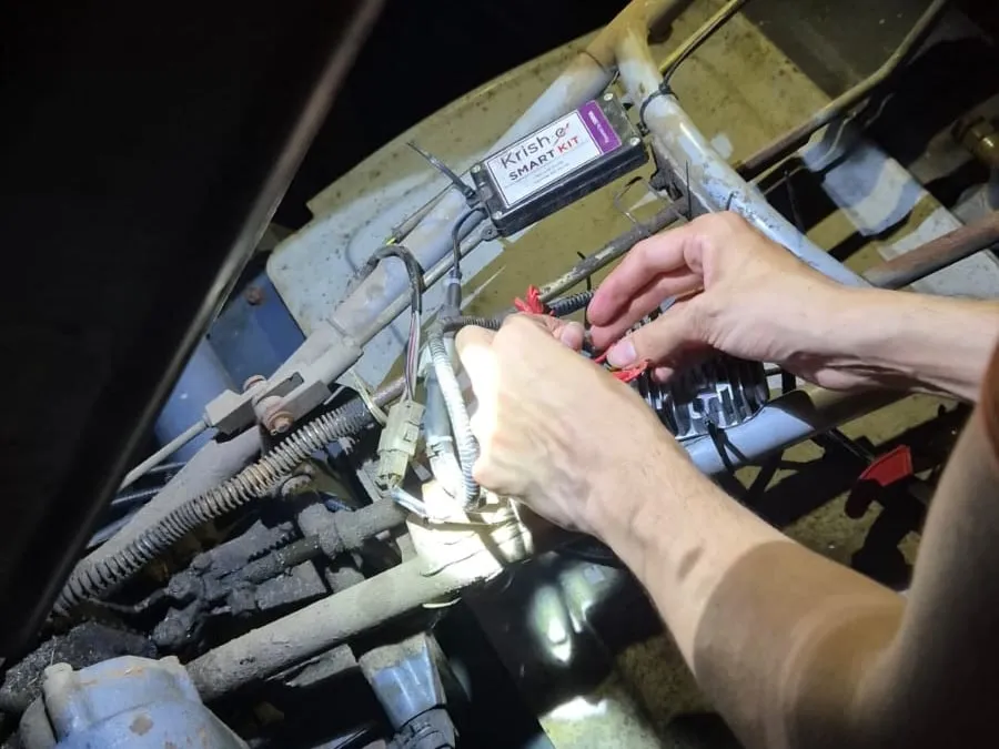Installing a Krish-e Smart Kit on a tiller, after dark.

Three parts of my work at Carnot deserve their own write-ups:

• Building an Analytics Stack with DuckDB, H3, and SQLMesh: large Parquet datasets, reusable spatial representations, and turning exploratory analysis into pipelines and dashboards.
• Watching Sugarcane Grow from Space: Optical Imagery, SAR, and Harvest Detection: using satellite imagery to detect harvests, and Synthetic Aperture Radar (SAR) for cloudy monsoon months.
• Can You Ask Your Data Questions in Plain English?: an LLM prototype that turned natural-language questions into validated SQL queries and charts.